Characterizing polymer material properties for automotive applications

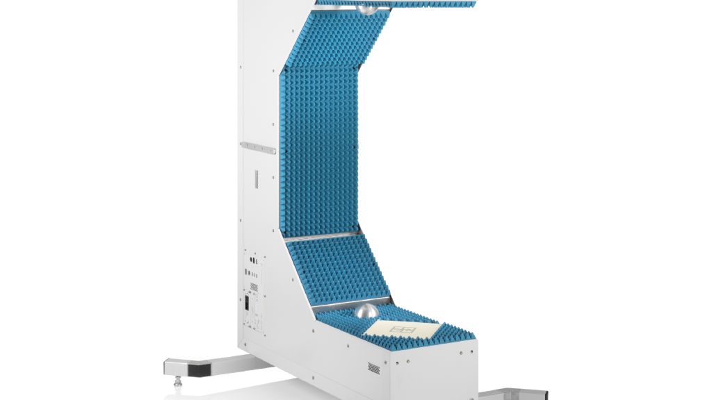
Automotive radar sensors concealed in bumpers must transmit in the correct frequency domain. To hide the sensors, radar-transparent areas are usually painted the same as the rest of the vehicle. You need to know bumper material propertiers when selecting paint and coatings. In the past, quasi-optical or waveguide based setups with vector network analyzers (VNA) were used. This application card describes a simplified material characterization method in the automotive radar frequency domain (76 GHz to 81 GHz) using the R&S®QAR50 automotive radome tester.

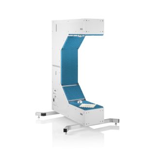
R&S®QAR50 automotive radome tester

Your task

Automotive bumpers usually have several layers: a structural base material, primer, paint and a clear coat. The structural base material is usually polypropylene (PP) or polycarbonate (PC) and gives a bumper its form. The base material is often the thickest layer but does not necessarily influence radar signals the most. The base layer can be adapted with various fillers that give it better UV resistance, rigidity, radar attenuation, etc. Primer is the second layer and helps paint adhere to the base material.

Primer layers are typically a couple of micrometers thick. Measuring the thickness of this layer and others can involve uncertainty.

The third layer is the paint applied to the primer. The thickness of the paint layer depends on the opacity of the paint but is usually very thin.

To protect paint from environmental influences, a clear coat is applied for the fourth and final layer.

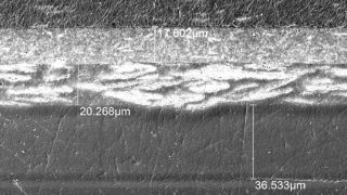
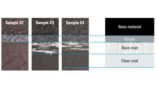
Estimating the electromagnetic properties of a bumper requires precise information about the thickness of each layer. A scanning electron microscope can determine their thickness (see Fig. 1).

Fig. 1: Micrograph showing the different layers of an automotive bumper sample: base material (PP), primer, paint, clear coat (top to bottom).
Open Lightbox

All layers must be characterized independently. The following description uses four different samples to characterize all four layers:

  • First, just the base material is analyzed
  • Second, the primer is applied to the characterized base material and analyzed
  • The third and fourth steps follow the same logic of applying the next layer to the previous one

The sample must be destroyed to create the microgram. All the measurements above must be made beforehand. The following section examines the required RF analysis of the samples.

Rohde & Schwarz solution

Permittivity estimation with the R&S®QAR50

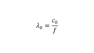
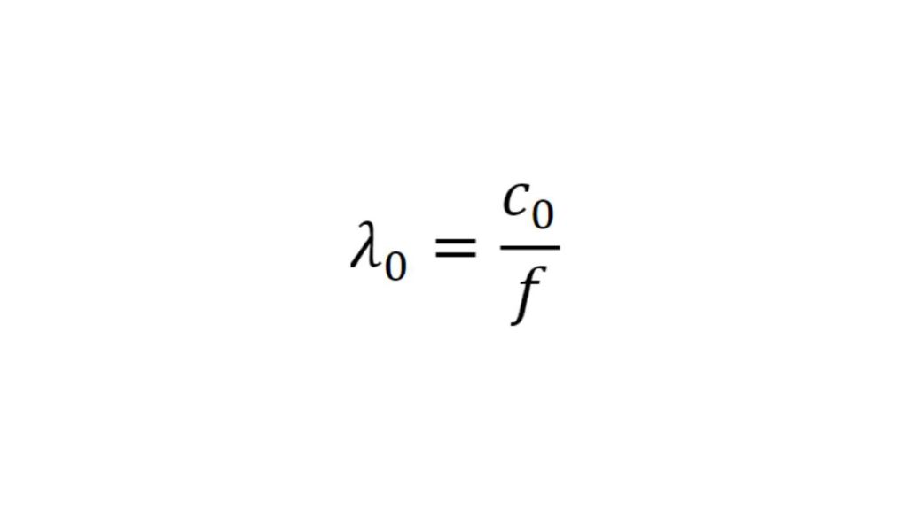
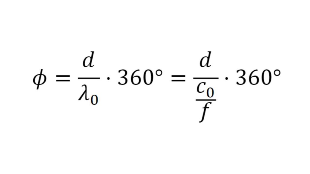
The permittivity of a sample determines the speed that electromagnetic waves move through a material and how the wave propagation is slowed. Reducing the speed of the electromagnetic wave reduces the wavelength inside the material. With frequency f and speed of light c0 in a vacuum, the wavelength λ0 is defined as:

Formel 1

Typical automotive radar frequency: fradar = 76.5 GHz, wavelength: λ0 = 3.92 mm.

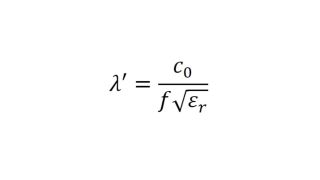
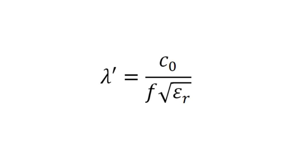
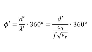
The wavelength inside a given material with the relative permittivity εr is calculated as:

Formel 2

Taking the sample polypropylene (PP) sheet with εr ~ 2.5, the wavelength in the PP sheet is calculated as λPP = 2.34 mm. Since the permittivity reduces the wavelength, it can be calculated using the measured phase if the thickness of the material under test (MUT) is known. The general procedure is demonstrated below.

Calculating permittivity with relative phase differences

The R&S®QAR50 is normalized to air propagation and every material positioned between the two clusters alters the phase at the receiving antennas. To characterize the sample, we want the phase difference stemming from the MUT within the measurement path.

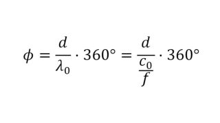
For reference, the phase Φ in degrees over distance d in free space is calculated as:

Formel 3

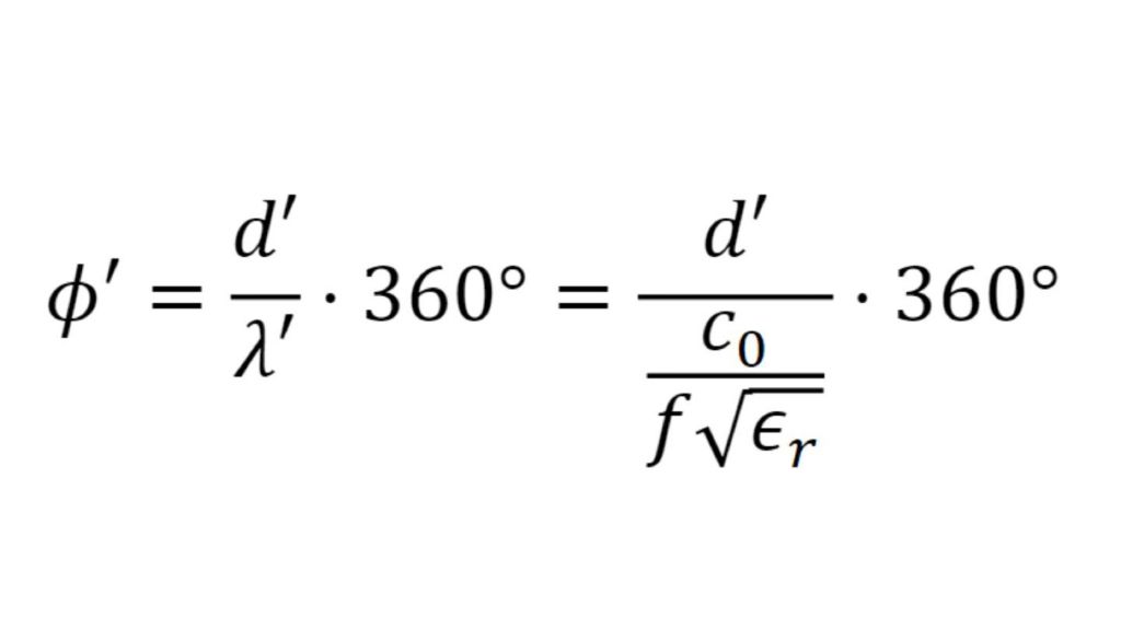
The phase Φ’ through material of thickness d’ is calculated as:

Formel 4

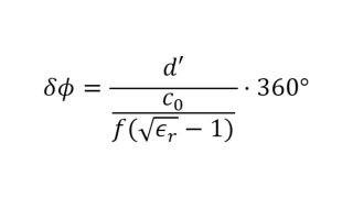
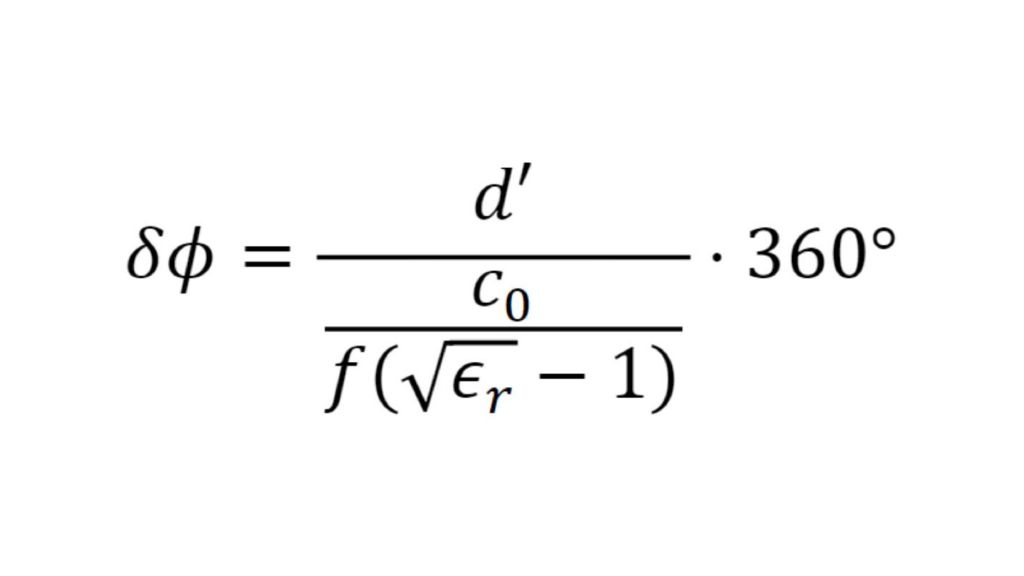
The δΦ phase change seen by the R&S®QAR50 is the difference between Φ and Φ’ equals:

Formel 5

A 2.92 mm PVC sheet with an estimated εr permittivity of approximately 2.5 will have an expected phase difference δΦ of nearly 158°.

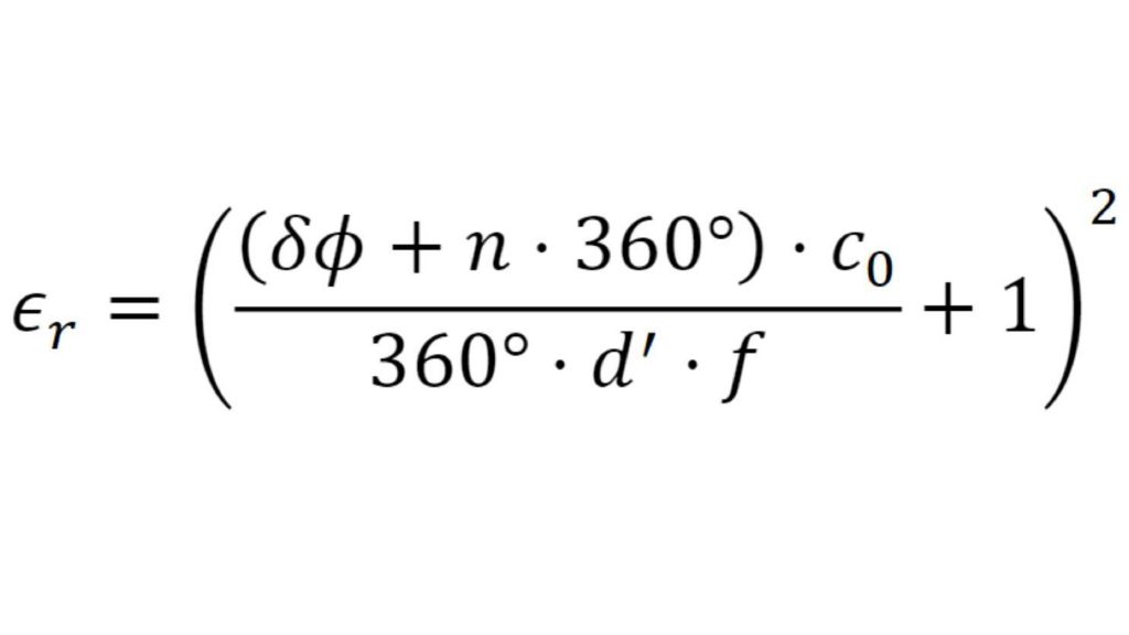
Since we are measuring the phase difference δΦ with the R&S®QAR50 and want to calculate permittivity εr, the formula above must be converted to:

Formel 6

The resulting permittivity is not unique since the phase difference could unknowingly be multiples of 360°. All possible solutions can be calculated for n Σ N0.

When a sample has multiple layers, all the layers except the one to be determined need to be characterized beforehand. Only then can the known layers be normalized out.

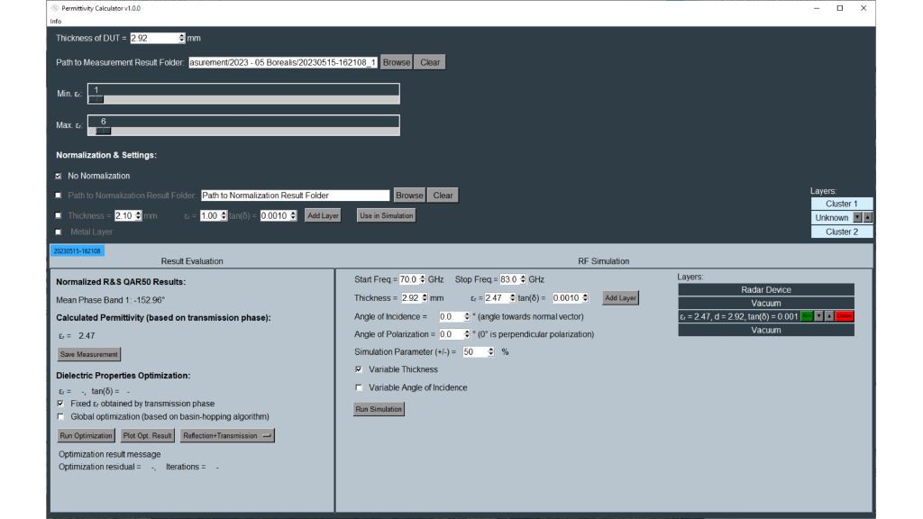
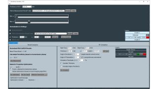
The R&S®QAR50 has software to simplify the calculations. The permittivity calculator utilizes precise phase measurement results from the R&S®QAR50 and can be seen in the example below.

Fig. 2: The base layer is loaded into the permittivity calculator. The calculated permittivity due to the phase change of approximately 153° at 76.5 GHz is εr = 2.47.
Open Lightbox

Sample characterization of a painted bumper sample

Using the same set of samples above, the thickness of the different layers is known and plates with individual layers are available for characterization. See Fig. 1 for the thickness of the individual layers.

Fig. 3: Adding normalization layers to characterize the primer, paint and clear coat
Open Lightbox

The base PP plate has a thickness of 2.92 mm for a measured phase difference of around –153° at 76.5 GHz. Using the measurement results as input parameters, the tool calculates an εr = 2.47 for that specific plate. Fig. 2 shows the result of the calculation in the software.

Using the RF calculation tool described below, the optimal thickness dopt can be derived from the minima for reflection and transmission loss. The reflection minima correlate to the sample resonance frequency and occur at multiples of half the wavelength within the material:

To characterize the remaining layers, the base material must be normalized out. Since its material permittivity is now known, the primer plate can also be normalized.

A normalization layer is added in the software and the next measurement result is loaded.

Normalization can either use a previous measurement or have a layer with a defined thickness and permittivity added manually. In our example, the normalization layer has a thickness of 2.92 mm and εr = 2.47 is manually added and visualized on the right side of the tool. Based on the measured primer thickness (see Fig. 1) and the measured phase shift of 5.3° from the R&S®QAR50, the estimated permittivity for the primer is εr = 18.3. The result can be seen in Fig. 3.

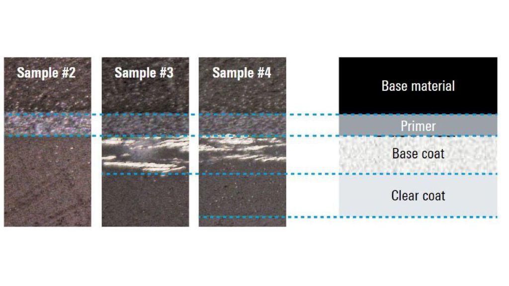
Fig. 4: Micrograph of the three processed samples
Fig. 4: Micrograph of the three processed samples showing significant differences in thickness of some layers. Sample #1 (raw PP) is not shown due to the different scaling.
Open Lightbox

As soon as the second layer is characterized, the remaining layers can be estimated using the steps described above. The characterized layers are added for normalization and the tool calculates the unknown permittivity.

Since the layer thicknesses across samples may differ, be careful when adding normalization layers. Fig. 4 shows the micrograph for the samples with an optical microscope. Significant differences in thickness of the paint layer can be spotted for the intermediate sample #3 (to characterize the paint) and sample #4 (to characterize the clear coat).

Result evaluation and RF simulation

Once a sample is loaded and characterized, the evaluation of the results and RF simulation areas at the bottom of the tool will appear and automatically be filled in with the plate-specific values.

“Normalized R&S®QAR50 results” shows the mean transmission phase across the selected sample evaluation area as measured by the R&S®QAR50. The transmission phase and thickness of the DUT are entered at the very top, the relative permittivity of the sample is calculated as described above. The R&S®QAR50 precisely measures the transmission phase but the calculated relative permittivity also depends on the accuracy of the thickness measurement.

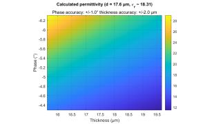
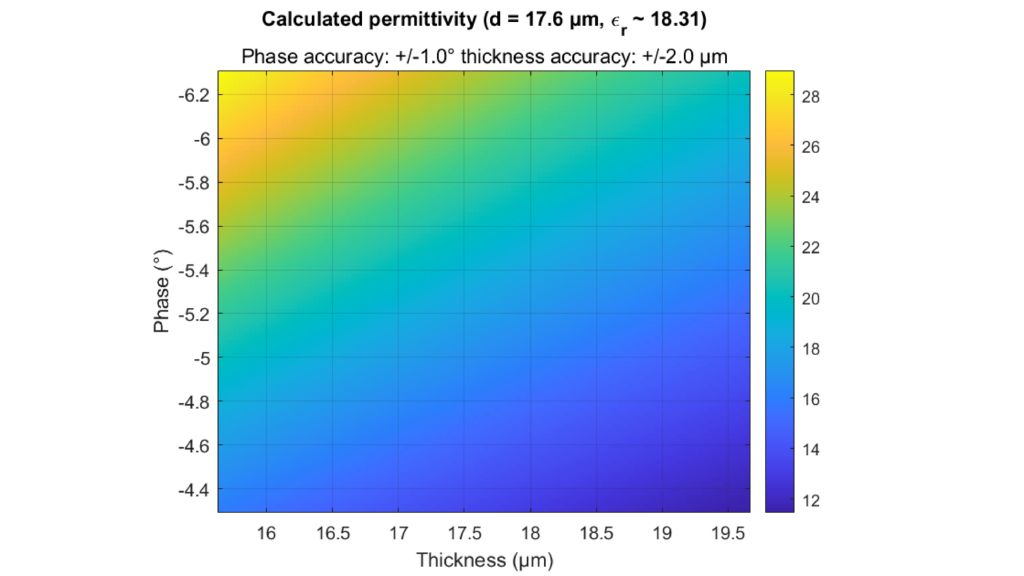
Fig. 5: Variation of relative permittivity calculation results with deviating thickness measurement and deviating phase measurement results illustrated for an exemplary coating.
Open Lightbox

Measurement inaccuracy influence
Be careful with thickness measurements since both values have an major influence on the calculated permittivity. Figs. 5 and 6 illustrate the impact of inaccurate thickness and/ or transmission phase measurements. Based on the measurements above, a coating with a thickness of d = 17.6 µm and a phase-shift of ∆φ = –5.3° results in permittivity with an εr of approximately 18.3. To illustrate the influence of inaccurate phase and thickness measurements, both parameters are evaluated over typical measurement accuracies: ±2 µm for the thickness measurement and ±1° for the transmission phase. Fig. 5 shows how the resulting calculated relative permittivity varies tremendously when measurement results become ever more inaccurate. Take care when measuring the RF characteristics of a material and when determining the thickness of the layers.

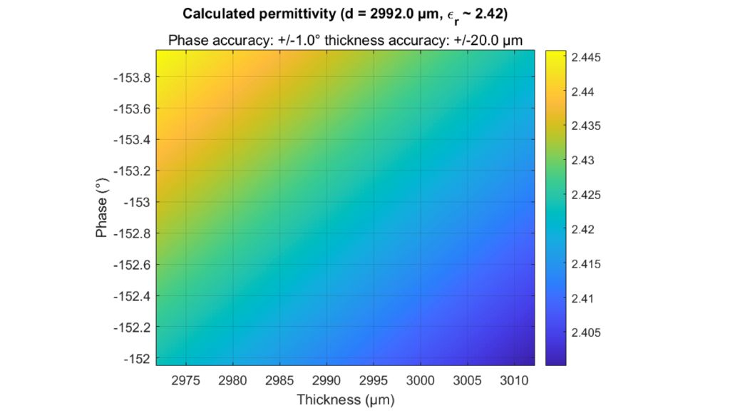
Fig. 6: Variation of relative permittivity calculation results with deviating thickness measurement and deviating phase measurement results illustrated for a sample substrate.
Open Lightbox

In Fig. 6, the sample substrate has a permittivity of 2.42 and a thickness of 2.92 mm. A micrometer was used for this thickness measurement and the measurement uncertainty is changed to ±20µm. The phase accuracy remains the identical since the same device was used for the measurement.

The effect is less significant for materials with lower permittivity and a thickness significantly larger than the measurement uncertainty (e.g. PC or PP).

Dielectric property optimization
The permittivity and the loss factor must be known to simulate material and material stacks and create a virtual duplicate of a radome. The relative permittivity εr correlates with the compression factor of the wavelength within the material, whereas the tan δ (loss factor) characterizes the specific attenuation of a transmitted signal from the layer.

The Rohde & Schwarz permittivity calculator can be used for both parameters and is ideal for radome layer simulations.

The tools for dielectric property estimation are in the lower left corner of the permittivity calculator software. The calculator uses an optimizer to find the best fit between measured and calculated frequency responses based on permittivity and loss factors. Users can choose between different calculation methods by checking:

  • “Fixed εr obtained by transmission phase” optimizes only tan δ while relative permittivity remains fixed
  • Unchecked, the optimizer has more freedom to improve relative permittivity; the relative permittivity calculated from the transmission phase acts as the initial value

Both methods have similar results for most materials. The transmission phase can be measured very accurately and is always a good point to start optimization.

“Optimize using logarithmic scale (dB)” sets the optimizer to work with a logarithmic curve to increase estimation accuracy for materials with resonance inside the R&S®QAR50 frequency band.

Global optimization uses multiple, randomly distributed starting points close to the calculated permittivity value to avoid optimizing into a local minimum.

The reflection curves from cluster 1 (S11) or cluster 2 (S22) are available for customer-specific applications.

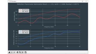
Fig. 7: Optimization results with fixed permittivity value
Open Lightbox

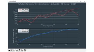
The measured and calculated frequency responses can be plotted after running the optimization. The “Plot Opt. Results” function plots the frequency response for the measured material (continuous line) as well as the virtual material (dotted line) using previously calculated material properties. Operators must check the validity of results for both methods. Figs. 7 and 8 show the generated graphs. Fig. 7 was created using the fixed permittivity from the transmission phase. Fig. 8 was created by optimizing both permittivity and loss tangents for the most suitable frequency response.
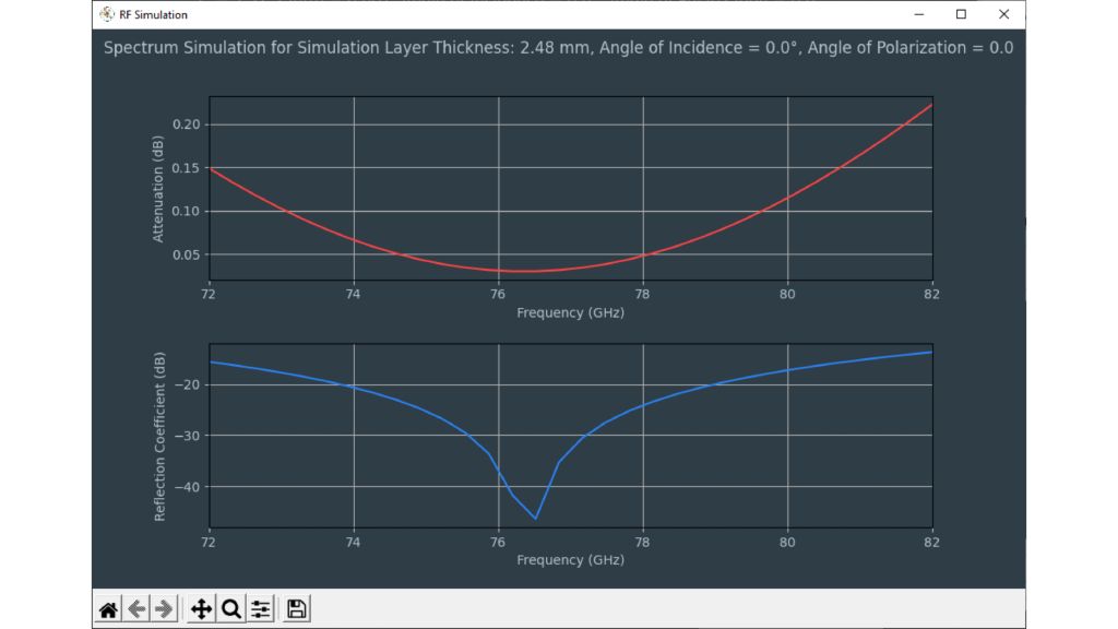
Fig. 8: Optimization results with optimized permittivity and loss factor
Open Lightbox

The material previously measured with the R&S®QAR50 is used as an example to estimate the loss factor.

As a general guideline, the residual optimization error is shown in the plot. The lower the error, the better the fitting. Optimizing both permittivity and loss factor are slightly more suitable for our example. The evaluation results can be used for simulations in the layer optimization tool.

Fig. 9: RF simulation result of a material sheet with εr = 2.51 and tan δ = 0.0012
Open Lightbox
Layer optimization tool

The layer optimization tool on the right side of the permittivity calculator is activated with the loading of a valid R&S®QAR50 measurement. The tool helps simulate multiple layers of paint and evaluate the effect of any differences in layer thickness.

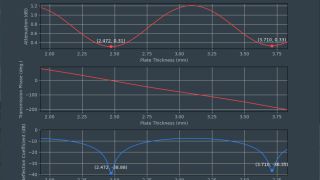
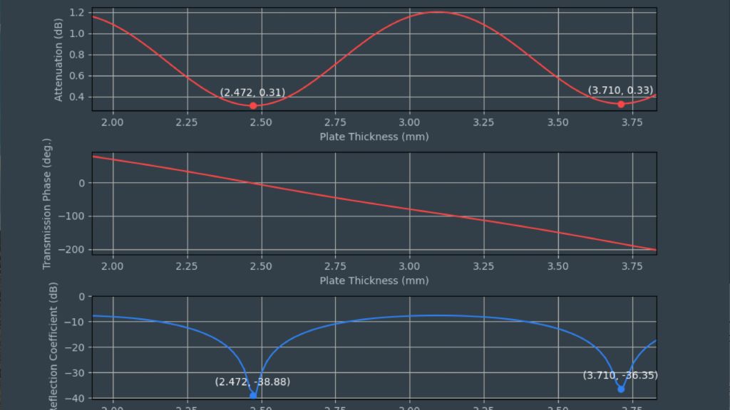
Start and stop frequencies represent radar bands used for an application. A digital twin of a part is created with the previously recorded material parameters for a single layer sheet. The “calculate optimal thickness” button can be used for an RF simulation of the layers. The calculation results for the sample material and thickness can be seen in Fig. 9

In Fig. 9 the optimal thickness for a single layer sheet is 2.47 mm. The thickness applies to unpainted radar covers. For simplicity’s sake, assume a single layer has been applied to the base material instead of three layers (primer, paint and coating). The added layer is d = 20 µm thick and has an εr = 15 with a tan δ = 0.02. The layer represents a typical paint used in the automotive industry.

Fig.10: Simulation of the sheet with an additional layer of paint
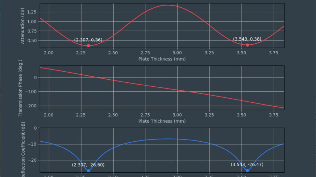
Fig. 10: Simulation of the sheet with an additional layer of paint (d = 20 μm, εr = 15 and tan δ = 0.02
Open Lightbox

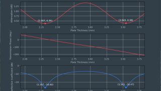
The challenge is still the same: We want an optimal base material thickness for one layer of paint. After adding the layer to the RF simulation tool, we can perform the same calculations as in Fig. 9. Assume the thickness of the paint layer is fixed and the optimal thickness for the base layer is needed. Fig. 10 shows the RF simulation result.

Fig. 11: Frequency response of a simulated layer with relative permittivity 2.5 and 2.48 mm thickness.
Open Lightbox

The layer has high permittivity and a major influence on radar performance despite its thinness and the effect can be seen in the simulation. Instead of 2.47 mm for the unpainted sheet, 2.31 mm would be the ideal thickness.

The same procedure applies to all remaining layers and the thickness of the bumper (or other layers) can be optimized

Another useful feature can be activated by hovering over a specific thickness point in the plot and pressing “n”. This will create a frequency resolved plot for that specific thickness. The frequency range is user defined in the main window of the permittivity calculator.

Fig. 12: Simulation of typical installation angles of the previously discussed simplified radar cover
Open Lightbox

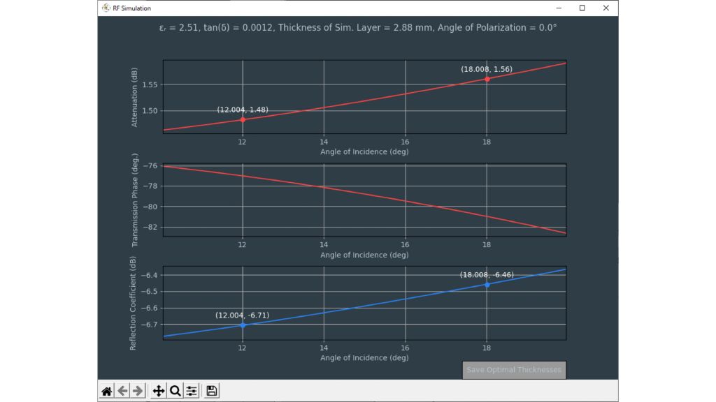
The simulation results described above can be calculated for varying thicknesses and simulation angles. Sticking with a simplified painted sheet, the installation angle of the cover relative to the radar impacts performance. The permittivity calculator software can be used to determine this effect.

Varying the installation angle from 10° to 20° (representing typical automotive installation angles) clearly reveals the effect of the incident angle.

The incidence angle and the polarization of the electric field relative to the incidence angle impact the optimal thickness and optimization. The permittivity calculator can be used to simulate the effects of the polarization angle of the incoming electromagnetic wave. 0° corresponds to a perpendicular polarization between the plane of incidence and the electric field of the incoming electric wave

Summary

When combined with the R&S®QAR50, the permittivity calculator is the ideal toolchain for over-the-air material characterization. Based on transmission loss, phase and reflection measurements, relative permittivity and the loss factor for the material under test can be calculated. Using the powerful RF simulation tool, the thickness of all layers can be adapted for a well-fitted radome in the automotive radar frequency range.

The permittivity calculator software can be downloaded for free from the R&S®QAR50 website:

www.rohde-schwarz.com/de/software/qar50/